Products / Technology

Entropy and spectral analysis

Two ideas do most of the work in our tools. Competitors use simple probability theory, no frequency analysis, and testability measures that ignore signal correlation.

01 — Information theory

Entropy

Entropy measures how much information a signal actually carries. A node that almost never changes carries very little — and a fault behind it is almost invisible to the tester.

We compute entropy through the design and place test points where they recover the most lost information per gate spent. That is why coverage reaches 99.98% on 0.71% additional chip area.

What it changes

01Test points are ranked by information gained, not by rough probability.

02Signal correlation is accounted for, so estimates hold on real designs.

03Fewer, better-placed points — shorter vectors and less added area.

Figure 01 — Entropy of a binary node

H(p) = −p log₂p − (1−p) log₂(1−p)

Entropy curve H(p) against p. The curve peaks at 1 when p is 0.5 and falls to 0 at both extremes; the low-entropy regions near p = 0 and p = 1 are outlined in red.

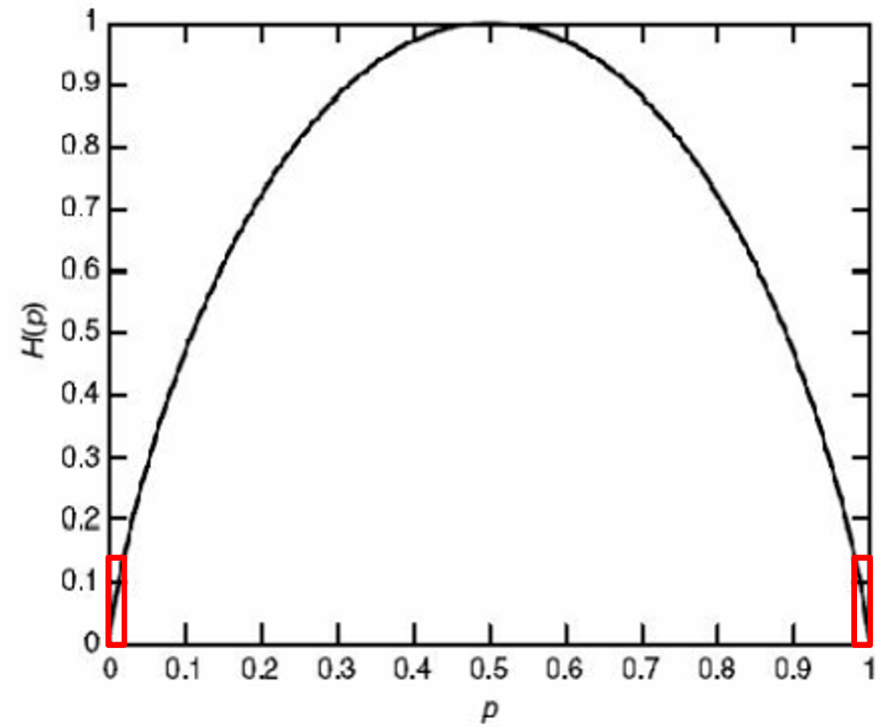
The regions outlined in red, near p = 0 and p = 1, are where entropy is lowest and faults hide. A node that sits at one value 95% of the time carries about a quarter of a bit. Test points are placed where they move a node back toward the peak, so each gate spent buys the most information.

Figure 01b — Entropy decides where a test point goes

Four AND levels, p(1) = 0.5 at the inputs

H ≥ 0.40 bits — observable H < 0.40 bits — information lost Traversing {{ curTxt }}

Node

p(1)

Entropy

Bits

Decision at {{ curTxt }}

Each AND gate squares the probability that its output is at logic 1, so information falls away with depth. The traversal reads entropy at every node and compares it against the threshold, marked by the dashed line on each bar: blue nodes are left alone, and the first red one takes the test point — which returns L3 to a full observable value without spending a second gate.

Stock photography.

02 — Digital frequency spectrum

Spectral analysis

Every internal signal has a spectrum: how fast it switches, and at which frequencies, as test patterns are applied.

Reading that spectrum tells us which parts of the design a pattern set can actually excite, and which faults it can never reach. It is also what makes path delay faults tractable — the fault model reliability now demands, and the one competitors find much harder to test for.

Applied in

Logic TPI — EntropyDFT^™ → RTL TPI, in development →

Figure 02 — Rademacher–Walsh basis

Eight Walsh functions w(n,x) on [0,1]

Every logic function can be written as a sum of these square waves. The transform reports how strongly a signal correlates with each one, and the sequency — the number of sign changes across the interval — is the frequency measure that ordinary Fourier analysis would give. Low-sequency energy means a node follows its inputs directly; energy in the high-sequency terms marks the correlated structure that hides faults, and that is where insertion pays.

Figure 03 — From circuit to spectrum

f = (a·b) + (b·c)

a b c = {{ patTxt }} f = {{ fTxt }} {{ stageTxt }}

Circuit under test

Output and its spectrum

Each pattern is applied at the inputs, propagated through the gates and observed at f. Correlating that output against the eight Walsh functions gives the spectrum below it: the b coefficient dominates at 6 of a possible 8, so b controls f far more than a or c do, and the second-order terms are what a probability-only measure would miss.

Want the mathematics applied to your design?

Enquire Now!